Monitoring Metrics #1: Visualizing the Variations in a Single Key Metric

In this first post in our “Monitoring Metrics” series, we’ll talk about the powerful ways you can monitor a single key metric in Anomalo.

Metrics are critical vital signs for modern data-driven companies. They can be leading indicators for company success, watched closely by the CEO and management team, and reported regularly to the board. Or they can be product, operational, or financial metrics that regularly inform important decisions made by teams.

In the modern data stack, teams have access to amazing data infrastructure for collecting and processing data for computing metrics. New business intelligence platforms make it easy to visualize, dashboard, and distribute metrics-based reporting. Now, companies like Airbnb are creating metrics layers that sit between the data warehouse and the reporting layers.

But all of this innovation in how metrics are computed and distributed can be undermined if the metrics themselves cannot be trusted. We need better systems for monitoring metrics that alert us when unexpected changes occur, and provide insight into why those changes were unusual.

In this post, we will cover:

• Monitoring a single metric
• Range-based monitoring
• Dynamic monitoring using a time series model
• Time series forecasts
• Exploring metrics visualizations in Anomalo

For now, we’ll focus on monitoring just one metric at a time. But in future posts, we will discuss how to effectively monitor metrics for multiple business segments, or even monitor large collections of metrics without being overwhelmed by false positive notifications.

Monitoring a single metric: taxi trip duration

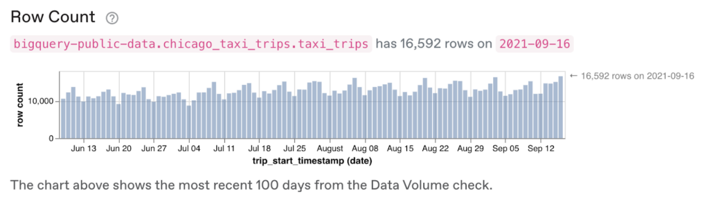
For this post, we will use publicly available data from Chicago Taxi trips stored in BigQuery. This view shows the row counts per day leading up to September 16th, 2021, which is near the last time that this data was updated:

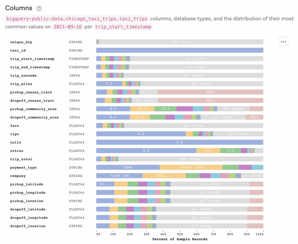
This view shows the columns in the table and their most common values:

In particular, let’s monitor how many minutes the average taxi trip takes in Chicago. We can define a trip_duration metric as:

trip_duration = avg(trip_seconds * 1.0 / 60)

If we were responsible for taxi trip times in Chicago, you can imagine that an automated or manual response might need to take place if this metric suddenly jumped or fell on a given day.

Range-based monitoring

The simplest form of metric monitoring would be to set a range for “normal” behavior for the metric, and alert if the metric deviates outside of this range. We could develop an estimate of the expected range by visualizing the trip_duration metric aggregated by day over a recent time period.

For example, based on the visualization below, we might expect the trip duration to always be above 16 minutes, but below 22 minutes:

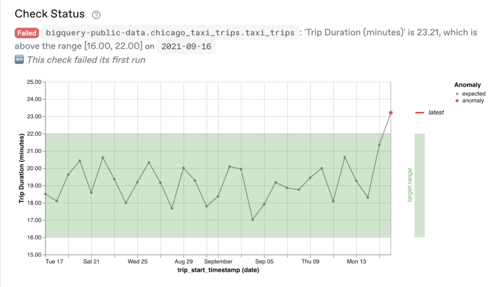
In the above visualization, you can see this target range (defined as [16.00, 22.00]), and that on 2021–09–16, the average duration shot up above this range to 23.21 minutes.

The challenge with this range-based approach to monitoring metrics is that the range is arbitrarily selected by a user. This should only be used when there is a hard and fast constraint on a metric that must not be violated (e.g., my home temperature should never be above 85° F or below 60° F).

In practice, we rarely have a strong intuition for what such constraints should be. So setting a range manually usually means that the range has to be frequently updated as:

• The metric drifts slowly outside of the expected range
• The metric varies seasonally by day of the week
• The metric varies seasonally during the course of a year
• The metric suddenly spikes or drops on holidays

However, if we have a history of data to compute for this metric, then we can solve many of the above problems by using a time series model.

Dynamic monitoring using a time series model

An effective time series model is able to evaluate a time series history of values for the key metric prior to the most recent date, and then predict an expected range for the most recent date. If the metric falls outside of the range, then there may be an anomaly worth investigating.

For example, here you can see a time series model fit for our trip_duration metric:

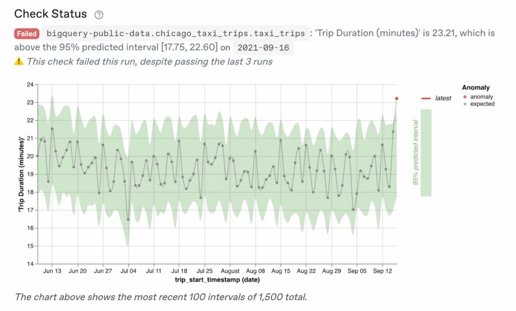
In particular, the time series model is predicting a range of [17.75, 22.60] for September 12, and the actual value of 22.21 is above that range.

A time-series model will ideally be able to adapt its predictions to fluctuations in the data caused by things like annual seasonality, day of the week, and slow data drift over time.

Time series forecasts

There are a variety of methods for producing time series forecasts:

• Traditional methods like exponential smoothing and ARIMA
• Additive approaches that decompose a time series into components
• Black box approaches such as recurrent neural networks

Each of these approaches have different tradeoffs, which merits a separate blog post! The best choice depends on the use case. For detecting anomalies in metrics, we care about the following:

• How accurate is the model at predicting the next observation in time?
• How well-calibrated are the confidence intervals produced? We want to be able to provide 95% confidence intervals over a robust benchmark of time series data sets.
• Can the model be easily explained and visualized?
• How robust is the model when presented with an unusual time series?
• How fast is the model at run time? In general, we try to keep the time series model run time below 20 seconds so that, when a human is running the check manually (at creation time, or when altering the configuration), they can get results back quickly.

At Anomalo, we found that the best results come from using additive approaches (such as those implemented in Prophet or GreyKite), with significant pre and post-processing of the time series data, guard rails for predictions, and extensive optimization of parameters.

Exploring single-metric visualizations in Anomalo

Now that we’ve explained how we do dynamic metric monitoring in Anomalo, let’s walk through the visualizations that let you really dig into the components of why a metric might be behaving abnormally—or just get insights from the data as a whole.

Forecast Zoom

When you create a “Key Metric” in Anomalo, the first detailed visualization we show is a Forecast Zoom plot. This allows the user to explore the full multi-year history of the time series and identifies any historical anomalies using the time series model:

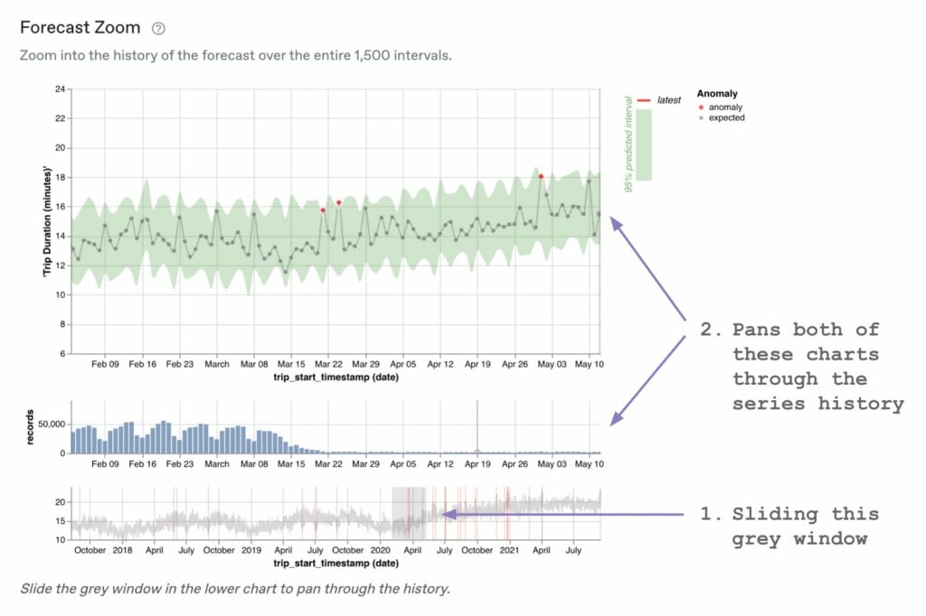
The top visualization is the metric series we’ve just looked at, with the fitted time series model visualized as a green confidence interval band behind the observations.

The middle visualization shows the row counts for each day supporting the metric in the chart above. This is important context, because there could be dates with very little data (which might have higher metric variance), or other distributional shifts that are important. In this case, we see that the number of rows dropped precipitously around March 15th, 2020, which is when the COVID-19 pandemic began in the US.

The final visualization on the bottom shows the time series (as a light grey line) over the entire five-year history. Anomalies in the time series are highlighted with vertical red lines. And the user can interact with the visualization by sliding the darker grey window to see the detailed visualizations for different periods of time.

The ability to zoom in and out on the historical time series data can lead to new insights about why the metric might be behaving a certain way. It’s also possible to go a level deeper and look not just at the overall forecast, but at its individual components.

Time Series Components

By looking at the time series components, you can examine each factor that drives variations in the time series, and look at its overall importance to the forecast.

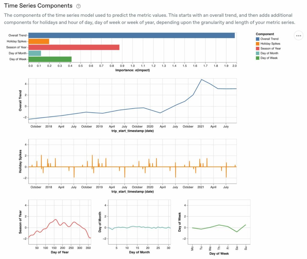
You can see here that the overall trend is by far the most important predictor, and there’s a major increase in average trip duration right around March 2020. This indicates that trips started to get much longer around the outbreak of the COVID-19 pandemic, hitting their peak in January 2021 before leveling off. Traveling in a taxi became much riskier at that time, and it stands to reason that people were likely to prefer longer trips when it was absolutely necessary, otherwise they might choose to walk or stay indoors.

We see that day of the year, the second most important component, indicates that taxi trip duration is at its highest in the summer and early fall, when school is out and people tend to take vacation. The holiday variation is interesting as well—on some holidays, we see shorter rides, and other holidays, longer rides.

Now, especially when you’re dealing with an anomalous metric, these explorations might still not be enough. You might want the ability to audit the forecast for the interval in question, which the next visualization can help with.

Forecast Explanation

In Anomalo, you can also get a “waterfall” chart that pieces out the components of the forecast for the most recent interval.

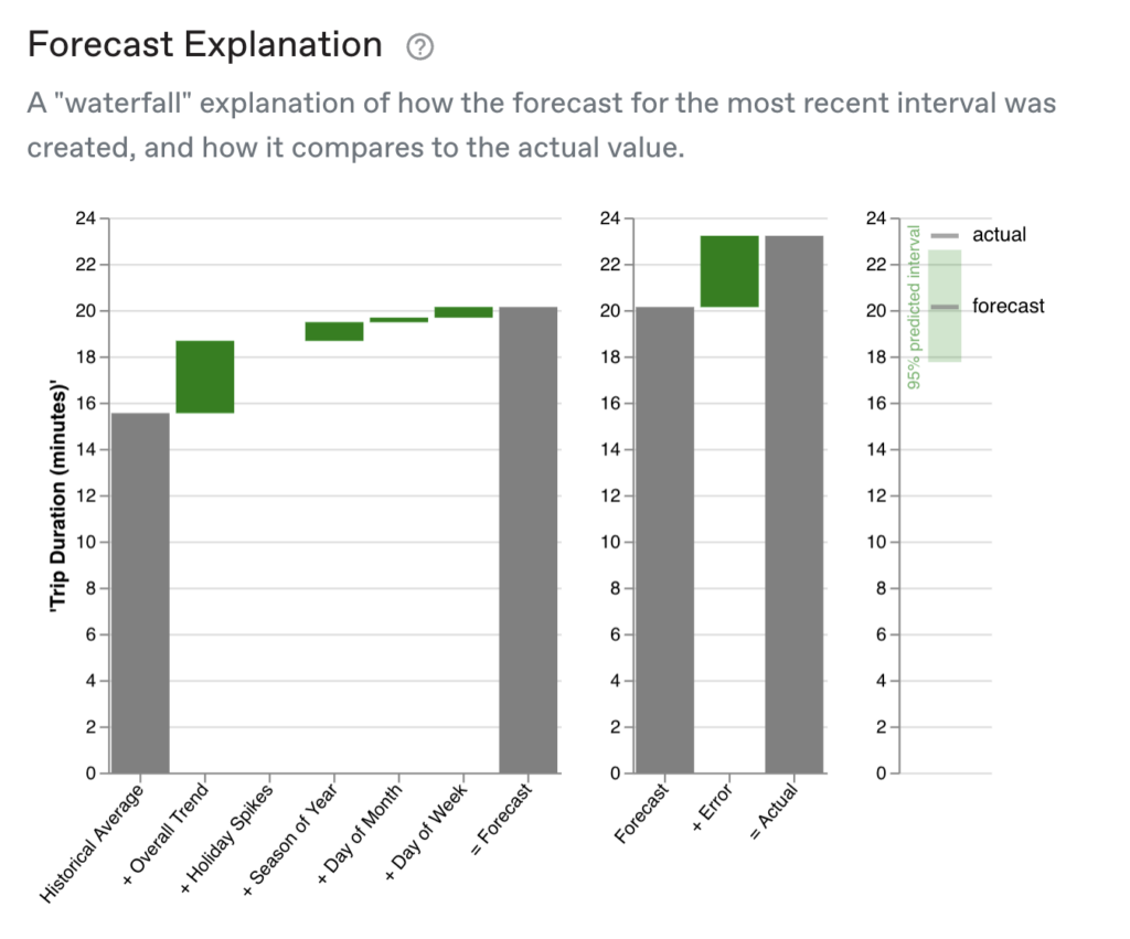
On the left, you can see that the time series took the historical average and added the contributions of the overall trend, holiday spikes (none in this case), season of year, day of week, and day of month to arrive at the final forecast. In this case, all the components bars are green, indicating that their contributions pushed the forecast up to a longer trip duration—often, you’ll see that some components are negative (red bars), pushing the forecast down.

On the right, you can see how much error, or difference, there is between the forecast and the actual metric. When the error is beyond the model’s confidence interval (where 95% of the points are predicted to fall inside that interval), an alert is triggered. We can see here that in this case, the actual metric was indeed anomalous, but not very much so, falling a few minutes outside of the model’s predicted range.

Wrapping it up

We’ve walked through what it means to monitor a single metric, and how you can do that using either a manually generated range or a dynamic time series model. We also explored a number of powerful visualizations that you can use to determine why a metric might be anomalous.

This is only the beginning of our metrics monitoring journey. In future posts, we’ll explain how to monitor business segments and collections of metrics. We’ll talk about how you can approach metrics that are constantly changing historically. And we’ll dig into the technical considerations for collecting data and training machine learning models. Stay tuned for more posts in this series on our blog!

‍